Simulating shunting performance is an important step in specifying the which shunt vehicle is right for our customers’ operations. Shunting simulations consider track properties such as gradients and curve radii as well as rolling stock characteristics such as length, mass and bearing resistance to make a prediction of the drawbar pull required to shunt the rolling stock through a given section of track.
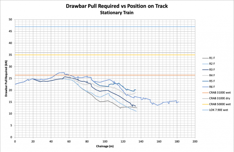
Most often performing these simulations the track properties are determined from vertical and horizontal alignment drawing of the track construction. From these Freightquip can construct a model that can predict the drawbar pull required for a given rolling stock configuration at any point on the track. The graph below shows one such simulation where the required drawbar pull in kilonewtons has been plotted against the chainage (or distance along the track).
Simulating from UTM coordinates
But what happens when you have a very large amount of track to simulate and you don’t have vertical alignment drawings for the track for which you want to simulate? In one such case a customer provided Freightquip with a file extracted from their GIS of their rail network. Fortunately, the GIS file used UTM coordinates which significantly simplified the process.
The first step in performing the simulation was to understand the data. The simplest way of doing this was to plot it out in a GIS system to visualise it. Upon viewing the data provided it was clear that this was going to be a big task, the data showed thousands of kilometres of track of which we were interested in a very small area of about 10 square kilometres.
To handle the large amount of data and quickly transform it into a usable dataset we utilised pandas, a data analysis library for Python, to quickly trim down the data to the area we were interested in and create dataframes to filter the data into individual track segments.
Now we had a much more manageable set of data cut into 30 track segments which we could use. There was still one problem how could we take these series of track segments of UTM coordinates and put them into a model where we needed curve radii? What was missing was a way to translate the track segments into a series of curves and straight segments.
The easiest way to identify the curves and straight sections in each track segment was to plot them out. This is where the UTM coordinates were very helpful as they could simply be plotted on an xy plane. After plotting out the track segments the straight sections and curved sections could be easily identified. This was done for each track segment.
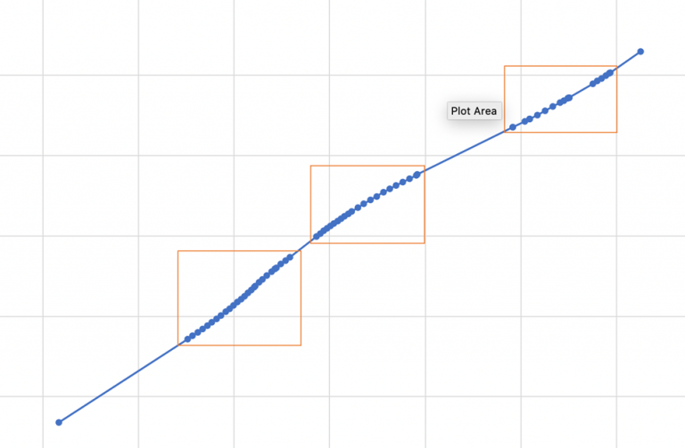
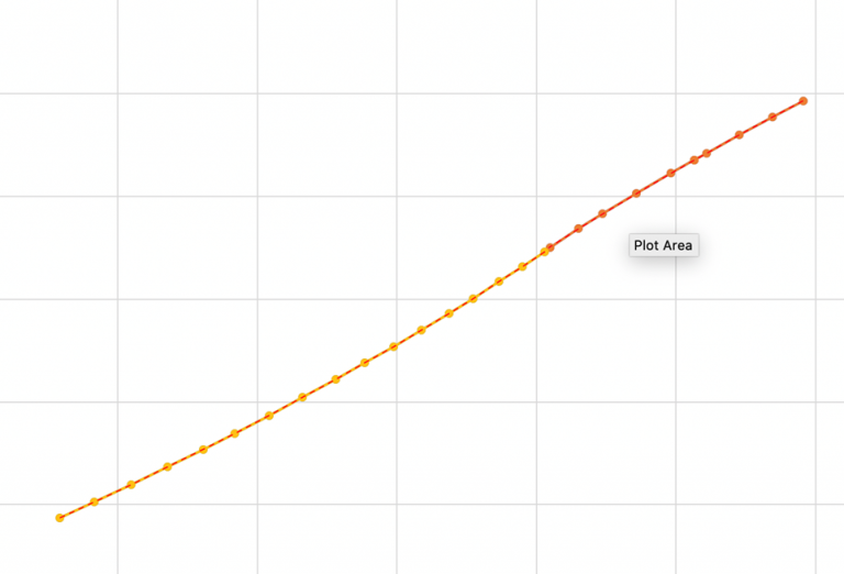
After plotting the track segments each of the curved sections was then further broken up into smaller segments around the curves as illustrated in Figure 2. These smaller segments were then plotted to identify individual curves. Often these smaller segments were composed of multiple curves as shown in Figure 3.
In railways the most common curve type are circular arcs, when sharp radius curves are required or for high-speed track transition curves can be employed. In this case however we could assume that each curve formed a circular arc.
Once we had identified the individual curves in the smaller segments the next task was to estimate their radii. This was done in two ways:
Firstly, a curve fitting algorithm took the points on the curve and an estimate of the centre point of the circle. As the distance between the centre point and any position on the arc is the same for all points, a least squares regression could be used to estimate the centre point and effective radius.
Secondly, using the least-squares regression the estimates could sometimes converge on an answer that didn’t quite fit the curve. To identify this more easily the estimated curve was plotted on the original curves, as shown by the red dotted line in Figure 3. The middle points in the curve and the estimated curve would have good agreement, if the radius of the estimated curve was too small or large it would diverge from the actual points at the ends of the curve. If the curve could be seen to diverge at the ends, the centre point was adjusted, and the curve fitting redone.
Now, after completing the curve fitting, we had all the data we needed to complete the simulation: chainage (distance along the track), curve radii, and gradients. The data could then be feed into our model to complete the shunting simulation.
As the local agent for the Global Railcar Mover Group, we are able to offer the most comprehensive range of shunting tractors into the Australian market, and we can determine the most appropriate to meet the application.
View the full range here: